Supernumerary tentacles and fitness parameters of the host and the tumors
Budding and supernumerary tentacles
Transmissible tumors dataset
donor_transN <- subset(donor_trans, donor_trans$abnormalities == "Normal")

models <- glmulti(buds_10 ~ donor * donor_status * receiver * diff_maxR * Tumors,
    data = donor_transN, level = 2, method = "h", crit = "aicc", fitfunction = "lm",
    pl = FALSE)

tmp <- weightable(models)
tmp2 <- tmp[tmp$aicc <= min(tmp$aicc) + 2, ]
tmp2

best_rt1 <- lm(buds_10 ~ 1 + donor + donor_status + receiver + Tumors + diff_maxR +
    receiver:donor_status + Tumors:receiver + Tumors:diff_maxR, data = donor_transN)

best_rt2 <- lm(buds_10 ~ 1 + donor + donor_status + receiver + Tumors + diff_maxR +
    receiver:donor_status + Tumors:donor_status + Tumors:receiver, data = donor_transN)

best_rt3 <- lm(buds_10 ~ 1 + donor + donor_status + receiver + Tumors + diff_maxR +
    receiver:donor_status + Tumors:donor_status + Tumors:receiver + Tumors:diff_maxR,
    data = donor_transN)

best_rt4 <- lm(buds_10 ~ 1 + donor + donor_status + receiver + Tumors + diff_maxR +
    donor_status:donor + receiver:donor_status + Tumors:receiver + Tumors:diff_maxR,
    data = donor_transN)

best_rt5 <- lm(buds_10 ~ 1 + donor + donor_status + receiver + Tumors + diff_maxR +
    receiver:donor_status + Tumors:receiver, data = donor_transN)

best_rt6 <- lm(buds_10 ~ 1 + donor + donor_status + receiver + Tumors + diff_maxR +
    receiver:donor_status + Tumors:donor_status + Tumors:receiver + donor:diff_maxR,
    data = donor_transN)

tab_model(best_rt1, best_rt2, best_rt3, best_rt4, best_rt5, best_rt6, show.intercept = F)
It appears that the appearance of tumors in certain receivers and the
interaction of recipient and donor status are the factors influencing
the most the number of buds produced. However, the number of tentacles
also seems to play a role that cannot be ruled out. To focus the
analysis on our parameters of interest, we will create groups of donors
and recipients to analyze the general relationship between tentacle
number and budding at the intra-group level.
Intra-group analysis
donor_transN$groupDR <- paste0(donor_transN$donor, donor_transN$donor_status, donor_transN$receiver)

best_rt10.4 <- lmer(buds_10 ~ 1 + diff_maxR * Tumors + (1 | groupDR), data = donor_transN)
best_rt10.3 <- lmer(buds_10 ~ 1 + diff_maxR + Tumors + (1 | groupDR), data = donor_transN)
best_rt10.2 <- lmer(buds_10 ~ 1 + diff_maxR + (1 | groupDR), data = donor_transN)
best_rt10.1 <- lmer(buds_10 ~ 1 + Tumors + (1 | groupDR), data = donor_transN)
best_rt10.0 <- lmer(buds_10 ~ 1 + (1 | groupDR), data = donor_transN)

AICc(best_rt10.4, best_rt10.3, best_rt10.2, best_rt10.1, best_rt10.0)
## df AICc
## best_rt10.4 6 648.2747
## best_rt10.3 5 653.0875
## best_rt10.2 4 660.7359
## best_rt10.1 4 673.5175
## best_rt10.0 3 678.8187
Table of the results of the best fitted models (lower AICc+2)
| buds_10 | buds_10 | buds_10 | buds_10 | buds_10 | |||||||||||
|---|---|---|---|---|---|---|---|---|---|---|---|---|---|---|---|
| Predictors | Estimates | CI | p | Estimates | CI | p | Estimates | CI | p | Estimates | CI | p | Estimates | CI | p |
| diff maxR | 2.99 | 0.71 – 5.27 | 0.011 | 0.71 | -0.33 – 1.76 | 0.179 | 0.36 | -0.68 – 1.40 | 0.498 | ||||||
| Tumors [1] | -3.08 | -7.40 – 1.24 | 0.160 | -5.29 | -9.19 – -1.38 | 0.009 | -4.02 | -7.72 – -0.32 | 0.033 | ||||||
| diff maxR × Tumors [1] | -2.75 | -5.21 – -0.29 | 0.029 | ||||||||||||
| Random Effects | |||||||||||||||
| σ2 | 58.63 | 60.95 | 63.37 | 60.53 | 61.64 | ||||||||||
| τ00 | 19.45 groupDR | 21.64 groupDR | 33.02 groupDR | 24.18 groupDR | 32.80 groupDR | ||||||||||
| ICC | 0.25 | 0.26 | 0.34 | 0.29 | 0.35 | ||||||||||
| N | 8 groupDR | 8 groupDR | 8 groupDR | 8 groupDR | 8 groupDR | ||||||||||
| Observations | 92 | 92 | 92 | 95 | 95 | ||||||||||
| Marginal R2 / Conditional R2 | 0.115 / 0.335 | 0.072 / 0.315 | 0.004 / 0.345 | 0.044 / 0.317 | 0.000 / 0.347 | ||||||||||
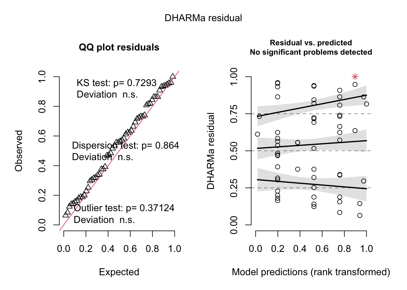
simulateResiduals(best_rt10.4, plot = T)
Final model results:
tab_model(best_rt10.4, show.intercept = F)| buds_10 | |||
|---|---|---|---|
| Predictors | Estimates | CI | p |
| diff maxR | 2.99 | 0.71 – 5.27 | 0.011 |
| Tumors [1] | -3.08 | -7.40 – 1.24 | 0.160 |
| diff maxR × Tumors [1] | -2.75 | -5.21 – -0.29 | 0.029 |
| Random Effects | |||
| σ2 | 58.63 | ||
| τ00 groupDR | 19.45 | ||
| ICC | 0.25 | ||
| N groupDR | 8 | ||
| Observations | 92 | ||
| Marginal R2 / Conditional R2 | 0.115 / 0.335 | ||
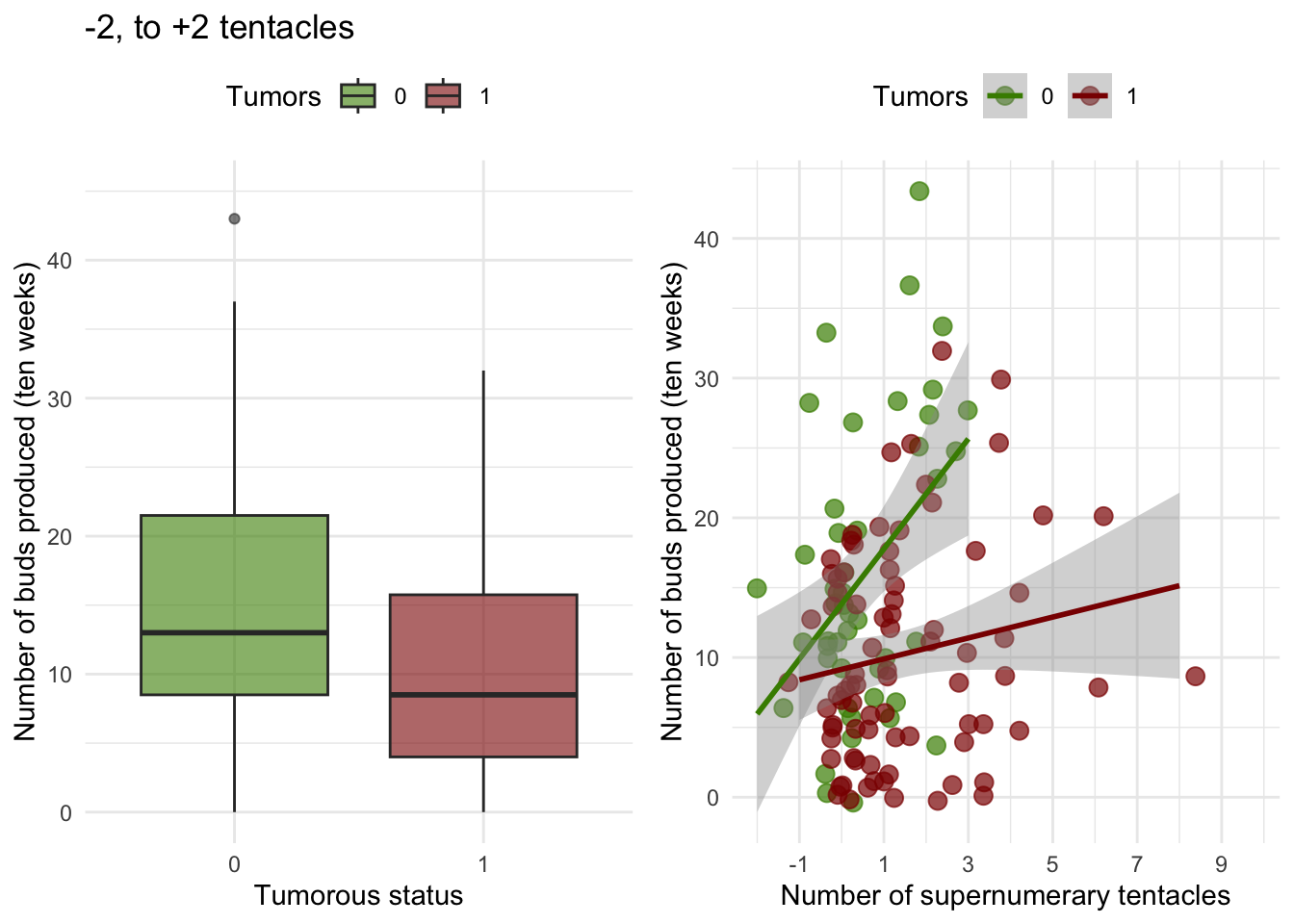
If we look at the intra-group level, the number of supernumerary
tentacles and the presence of tumors interact significantly to explain
the budding rate.
When does this relationship establish ?
best_rt10 <- lmer(buds_10 ~ 1 + tenta_10 * Tumors + (1 | groupDR), data = donor_transN)
best_rt9 <- lmer(buds_9 ~ 1 + tenta_9 * Tumors + (1 | groupDR), data = donor_transN)
best_rt8 <- lmer(buds_8 ~ 1 + tenta_8 * Tumors + (1 | groupDR), data = donor_transN)
best_rt7 <- lmer(buds_7 ~ 1 + tenta_7 * Tumors + (1 | groupDR), data = donor_transN)
best_rt6 <- lmer(buds_6 ~ 1 + tenta_6 * Tumors + (1 | groupDR), data = donor_transN)
best_rt5 <- lmer(buds_5 ~ 1 + tenta_5 * Tumors + (1 | groupDR), data = donor_transN)
best_rt4 <- lmer(buds_4 ~ 1 + tenta_4 * Tumors + (1 | groupDR), data = donor_transN)
best_rt3 <- lmer(buds_3 ~ 1 + tenta_3 * Tumors + (1 | groupDR), data = donor_transN)
best_rt2 <- lmer(buds_2 ~ 1 + tenta_2 * Tumors + (1 | groupDR), data = donor_transN)
best_rt1 <- lmer(buds_1 ~ 1 + tenta_1 * Tumors + (1 | groupDR), data = donor_transN)
tab_model(best_rt10, best_rt9, best_rt8, best_rt7, best_rt6, best_rt5, best_rt4,
best_rt3, best_rt2, best_rt1, show.intercept = F)| buds_10 | buds_9 | buds_8 | buds_7 | buds_6 | buds_5 | buds_4 | buds_3 | buds_2 | buds_1 | |||||||||||||||||||||
|---|---|---|---|---|---|---|---|---|---|---|---|---|---|---|---|---|---|---|---|---|---|---|---|---|---|---|---|---|---|---|
| Predictors | Estimates | CI | p | Estimates | CI | p | Estimates | CI | p | Estimates | CI | p | Estimates | CI | p | Estimates | CI | p | Estimates | CI | p | Estimates | CI | p | Estimates | CI | p | Estimates | CI | p |
| tenta 10 | 4.87 | 1.98 – 7.75 | 0.001 | |||||||||||||||||||||||||||
| Tumors [1] | 20.45 | 3.48 – 37.42 | 0.019 | 11.30 | 1.36 – 21.24 | 0.026 | 10.62 | 0.07 – 21.18 | 0.049 | 15.78 | 6.99 – 24.58 | 0.001 | 5.23 | -3.13 – 13.58 | 0.218 | 3.78 | -1.89 – 9.46 | 0.189 | 3.65 | -0.86 – 8.15 | 0.112 | 0.53 | -3.37 – 4.42 | 0.789 | -0.12 | -2.25 – 2.00 | 0.908 | -0.66 | -1.88 – 0.56 | 0.289 |
| tenta 10 × Tumors [1] | -4.57 | -7.58 – -1.56 | 0.003 | |||||||||||||||||||||||||||
| tenta 9 | 2.93 | 1.38 – 4.49 | <0.001 | |||||||||||||||||||||||||||
| tenta 9 × Tumors [1] | -2.68 | -4.43 – -0.94 | 0.003 | |||||||||||||||||||||||||||
| tenta 8 | 2.62 | 0.96 – 4.28 | 0.002 | |||||||||||||||||||||||||||
| tenta 8 × Tumors [1] | -2.23 | -4.04 – -0.42 | 0.016 | |||||||||||||||||||||||||||
| tenta 7 | 3.30 | 1.93 – 4.68 | <0.001 | |||||||||||||||||||||||||||
| tenta 7 × Tumors [1] | -3.16 | -4.69 – -1.62 | <0.001 | |||||||||||||||||||||||||||
| tenta 6 | 1.45 | 0.16 – 2.75 | 0.028 | |||||||||||||||||||||||||||
| tenta 6 × Tumors [1] | -1.12 | -2.61 – 0.36 | 0.136 | |||||||||||||||||||||||||||
| tenta 5 | 0.91 | 0.05 – 1.77 | 0.038 | |||||||||||||||||||||||||||
| tenta 5 × Tumors [1] | -0.77 | -1.77 – 0.22 | 0.128 | |||||||||||||||||||||||||||
| tenta 4 | 0.90 | 0.27 – 1.53 | 0.006 | |||||||||||||||||||||||||||
| tenta 4 × Tumors [1] | -0.72 | -1.48 – 0.05 | 0.066 | |||||||||||||||||||||||||||
| tenta 3 | 0.37 | -0.21 – 0.95 | 0.210 | |||||||||||||||||||||||||||
| tenta 3 × Tumors [1] | -0.14 | -0.82 – 0.55 | 0.699 | |||||||||||||||||||||||||||
| tenta 2 | -0.03 | -0.33 – 0.28 | 0.861 | |||||||||||||||||||||||||||
| tenta 2 × Tumors [1] | 0.04 | -0.34 – 0.42 | 0.846 | |||||||||||||||||||||||||||
| tenta 1 | -0.05 | -0.22 – 0.12 | 0.575 | |||||||||||||||||||||||||||
| tenta 1 × Tumors [1] | 0.14 | -0.07 – 0.36 | 0.189 | |||||||||||||||||||||||||||
| Random Effects | ||||||||||||||||||||||||||||||
| σ2 | 56.37 | 46.86 | 41.98 | 29.99 | 24.69 | 15.82 | 9.96 | 4.84 | 1.62 | 0.37 | ||||||||||||||||||||
| τ00 | 15.35 groupDR | 19.27 groupDR | 14.62 groupDR | 6.05 groupDR | 6.05 groupDR | 3.66 groupDR | 1.37 groupDR | 0.94 groupDR | 0.40 groupDR | 0.08 groupDR | ||||||||||||||||||||
| ICC | 0.21 | 0.29 | 0.26 | 0.17 | 0.20 | 0.19 | 0.12 | 0.16 | 0.20 | 0.18 | ||||||||||||||||||||
| N | 8 groupDR | 8 groupDR | 8 groupDR | 8 groupDR | 8 groupDR | 8 groupDR | 8 groupDR | 8 groupDR | 8 groupDR | 8 groupDR | ||||||||||||||||||||
| Observations | 95 | 91 | 111 | 116 | 125 | 138 | 146 | 147 | 152 | 154 | ||||||||||||||||||||
| Marginal R2 / Conditional R2 | 0.149 / 0.331 | 0.126 / 0.381 | 0.079 / 0.317 | 0.164 / 0.304 | 0.040 / 0.229 | 0.031 / 0.213 | 0.053 / 0.168 | 0.018 / 0.177 | 0.001 / 0.201 | 0.024 / 0.204 | ||||||||||||||||||||
The relationship between the number of tentacles, the tumor presence,
and the budding seems to appear only after the third week, corresponding
to the establishment of the tumorous phenotype and the increase in the
number of tentacles.
Spontaneaous tumors dataset
donor_spontN <- subset(donor_spont, donor_spont$abnormalities == "Normal")

models <- glmulti(buds_10 ~ donor * donor_status * receiver * diff_maxR * Tumors,
    data = donor_spontN, level = 2, method = "h", crit = "aicc", fitfunction = "lm",
    pl = FALSE)

tmp <- weightable(models)
tmp2 <- tmp[tmp$aicc <= min(tmp$aicc) + 2, ]
tmp2

best_rt1 <- lm(buds_10 ~ 1 + donor + receiver + Tumors + diff_maxR + receiver:donor +
    Tumors:donor + donor_status:diff_maxR, data = donor_spontN)

best_rt2 <- lm(buds_10 ~ 1 + donor + receiver + Tumors + diff_maxR + receiver:donor +
    Tumors:donor + donor_status:diff_maxR + receiver:diff_maxR, data = donor_spontN)

best_rt3 <- lm(buds_10 ~ 1 + donor + receiver + diff_maxR + receiver:donor + donor:diff_maxR +
    donor_status:diff_maxR, data = donor_spontN)

best_rt4 <- lm(buds_10 ~ 1 + donor + donor_status + receiver + Tumors + diff_maxR +
    receiver:donor + Tumors:donor + donor_status:diff_maxR, data = donor_spontN)

best_rt5 <- lm(buds_10 ~ 1 + donor + donor_status + receiver + diff_maxR + receiver:donor +
    donor:diff_maxR + donor_status:diff_maxR, data = donor_spontN)

best_rt6 <- lm(buds_10 ~ 1 + donor + receiver + Tumors + diff_maxR + receiver:donor +
    Tumors:donor + donor_status:diff_maxR + Tumors:diff_maxR, data = donor_spontN)

best_rt7 <- lm(buds_10 ~ 1 + donor + receiver + Tumors + diff_maxR + receiver:donor +
    Tumors:donor + donor_status:diff_maxR + Tumors:diff_maxR, data = donor_spontN)

best_rt8 <- lm(buds_10 ~ 1 + donor + donor_status + receiver + Tumors + diff_maxR +
    donor_status:donor + receiver:donor + Tumors:donor + donor_status:diff_maxR,
    data = donor_spontN)
best_rt9 <- lm(buds_10 ~ 1 + donor + receiver + Tumors + diff_maxR + receiver:donor +
    Tumors:donor + donor:diff_maxR + donor_status:diff_maxR, data = donor_spontN)

tab_model(best_rt1, best_rt2, best_rt3, best_rt4, best_rt5, best_rt6, best_rt7, best_rt8,
    best_rt9, show.intercept = F)
It seems that the appearance of tumors in certain donors and the
interaction of recipient and donor are the factors influencing the most
the number of buds. The number of tentacles also seems to play a role
when the donor was tumorous. To focus the analysis on the parameters of
interest, we will create groups of donors and recipients.
Intra group analysis
donor_spontN$groupDR <- as.factor(paste0(donor_spontN$donor, donor_spontN$donor_status,
    donor_spontN$receiver))
summary(donor_spontN$groupDR)
## MTNTSpB MTNTTV MTTSpB MTTTV SpBNTSpB SpBNTTV SpBTSpB SpBTTV
## 6 10 7 9 19 28 10 6best_rt10.4 <- lmer(buds_10 ~ 1 + diff_maxR * Tumors + (1 | groupDR), data = donor_spontN)
best_rt10.3 <- lmer(buds_10 ~ 1 + diff_maxR + Tumors + (1 | groupDR), data = donor_spontN)
best_rt10.2 <- lmer(buds_10 ~ 1 + diff_maxR + (1 | groupDR), data = donor_spontN)
best_rt10.1 <- lmer(buds_10 ~ 1 + Tumors + (1 | groupDR), data = donor_spontN)
best_rt10.0 <- lmer(buds_10 ~ 1 + (1 | groupDR), data = donor_spontN)
AICc(best_rt10.4, best_rt10.3, best_rt10.2, best_rt10.1, best_rt10.0)## df AICc
## best_rt10.4 6 373.7325
## best_rt10.3 5 376.3829
## best_rt10.2 4 377.8042
## best_rt10.1 4 399.9832
## best_rt10.0 3 400.6056Table of the results of the best fitted models (lower AICc+2)
| buds_10 | buds_10 | buds_10 | buds_10 | buds_10 | |||||||||||
|---|---|---|---|---|---|---|---|---|---|---|---|---|---|---|---|
| Predictors | Estimates | CI | p | Estimates | CI | p | Estimates | CI | p | Estimates | CI | p | Estimates | CI | p |
| diff maxR | -1.59 | -5.37 – 2.19 | 0.402 | 0.83 | -0.60 – 2.25 | 0.248 | 0.64 | -0.73 – 2.01 | 0.352 | ||||||
| Tumors [1] | -2.29 | -5.84 – 1.25 | 0.200 | -1.64 | -5.09 – 1.81 | 0.346 | -0.62 | -3.80 – 2.56 | 0.697 | ||||||
| diff maxR × Tumors [1] | 2.79 | -1.25 – 6.83 | 0.172 | ||||||||||||
| Random Effects | |||||||||||||||
| σ2 | 29.43 | 30.04 | 30.20 | 29.18 | 28.83 | ||||||||||
| τ00 | 20.67 groupDR | 20.23 groupDR | 18.91 groupDR | 20.26 groupDR | 19.60 groupDR | ||||||||||
| ICC | 0.41 | 0.40 | 0.39 | 0.41 | 0.40 | ||||||||||
| N | 8 groupDR | 8 groupDR | 8 groupDR | 8 groupDR | 8 groupDR | ||||||||||
| Observations | 58 | 58 | 58 | 62 | 62 | ||||||||||
| Marginal R2 / Conditional R2 | 0.040 / 0.436 | 0.021 / 0.415 | 0.010 / 0.391 | 0.002 / 0.411 | 0.000 / 0.405 | ||||||||||
tab_model(best_rt10.4, show.intercept = F)| buds_10 | |||
|---|---|---|---|
| Predictors | Estimates | CI | p |
| diff maxR | -1.59 | -5.37 – 2.19 | 0.402 |
| Tumors [1] | -2.29 | -5.84 – 1.25 | 0.200 |
| diff maxR × Tumors [1] | 2.79 | -1.25 – 6.83 | 0.172 |
| Random Effects | |||
| σ2 | 29.43 | ||
| τ00 groupDR | 20.67 | ||
| ICC | 0.41 | ||
| N groupDR | 8 | ||
| Observations | 58 | ||
| Marginal R2 / Conditional R2 | 0.040 / 0.436 | ||
If we look at the intra-group level, there is no clear relationship,
which is quite expected given the absence of an increased number of
tentacles when the donor was a spontaneous tumor.
When does this relationship establish ?
best_rt10 <- lmer(buds_10 ~ 1 + tenta_10 * Tumors + (1 | groupDR), data = donor_spontN)
best_rt9 <- lmer(buds_9 ~ 1 + tenta_9 * Tumors + (1 | groupDR), data = donor_spontN)
best_rt8 <- lmer(buds_8 ~ 1 + tenta_8 * Tumors + (1 | groupDR), data = donor_spontN)
best_rt7 <- lmer(buds_7 ~ 1 + tenta_7 * Tumors + (1 | groupDR), data = donor_spontN)
best_rt6 <- lmer(buds_6 ~ 1 + tenta_6 * Tumors + (1 | groupDR), data = donor_spontN)
best_rt5 <- lmer(buds_5 ~ 1 + tenta_5 * Tumors + (1 | groupDR), data = donor_spontN)
best_rt4 <- lmer(buds_4 ~ 1 + tenta_4 * Tumors + (1 | groupDR), data = donor_spontN)
best_rt3 <- lmer(buds_3 ~ 1 + tenta_3 * Tumors + (1 | groupDR), data = donor_spontN)
best_rt2 <- lmer(buds_2 ~ 1 + tenta_2 * Tumors + (1 | groupDR), data = donor_spontN)
best_rt1 <- lmer(buds_1 ~ 1 + tenta_1 * Tumors + (1 | groupDR), data = donor_spontN)

tab_model(best_rt10, best_rt9, best_rt8, best_rt7, best_rt6, best_rt5, best_rt4,
best_rt3, best_rt2, best_rt1, show.intercept = F)| buds_10 | buds_9 | buds_8 | buds_7 | buds_6 | buds_5 | buds_4 | buds_3 | buds_2 | buds_1 | |||||||||||||||||||||
|---|---|---|---|---|---|---|---|---|---|---|---|---|---|---|---|---|---|---|---|---|---|---|---|---|---|---|---|---|---|---|
| Predictors | Estimates | CI | p | Estimates | CI | p | Estimates | CI | p | Estimates | CI | p | Estimates | CI | p | Estimates | CI | p | Estimates | CI | p | Estimates | CI | p | Estimates | CI | p | Estimates | CI | p |
| tenta 10 | 0.94 | -2.33 – 4.21 | 0.568 | |||||||||||||||||||||||||||
| Tumors [1] | -6.84 | -23.33 – 9.64 | 0.409 | -6.17 | -17.01 – 4.67 | 0.259 | -3.51 | -15.38 – 8.36 | 0.557 | -1.71 | -11.55 – 8.14 | 0.730 | -6.97 | -15.84 – 1.91 | 0.122 | -2.05 | -8.39 – 4.28 | 0.521 | -1.84 | -5.94 – 2.26 | 0.375 | -1.02 | -4.99 – 2.95 | 0.610 | -1.22 | -3.57 – 1.13 | 0.305 | -0.23 | -1.66 – 1.20 | 0.748 |
| tenta 10 × Tumors [1] | 0.90 | -2.48 – 4.27 | 0.597 | |||||||||||||||||||||||||||
| tenta 9 | 0.04 | -1.86 – 1.94 | 0.967 | |||||||||||||||||||||||||||
| tenta 9 × Tumors [1] | 1.14 | -1.02 – 3.30 | 0.294 | |||||||||||||||||||||||||||
| tenta 8 | 0.33 | -1.77 – 2.44 | 0.752 | |||||||||||||||||||||||||||
| tenta 8 × Tumors [1] | 0.70 | -1.59 – 2.99 | 0.543 | |||||||||||||||||||||||||||
| tenta 7 | 0.83 | -0.72 – 2.37 | 0.289 | |||||||||||||||||||||||||||
| tenta 7 × Tumors [1] | 0.33 | -1.60 – 2.27 | 0.730 | |||||||||||||||||||||||||||
| tenta 6 | -0.26 | -1.91 – 1.39 | 0.756 | |||||||||||||||||||||||||||
| tenta 6 × Tumors [1] | 1.48 | -0.31 – 3.26 | 0.103 | |||||||||||||||||||||||||||
| tenta 5 | 0.50 | -0.64 – 1.64 | 0.384 | |||||||||||||||||||||||||||
| tenta 5 × Tumors [1] | 0.39 | -0.87 – 1.65 | 0.537 | |||||||||||||||||||||||||||
| tenta 4 | 0.44 | -0.02 – 0.90 | 0.060 | |||||||||||||||||||||||||||
| tenta 4 × Tumors [1] | 0.33 | -0.45 – 1.10 | 0.403 | |||||||||||||||||||||||||||
| tenta 3 | 0.28 | -0.40 – 0.95 | 0.414 | |||||||||||||||||||||||||||
| tenta 3 × Tumors [1] | 0.18 | -0.59 – 0.95 | 0.645 | |||||||||||||||||||||||||||
| tenta 2 | -0.05 | -0.40 – 0.29 | 0.765 | |||||||||||||||||||||||||||
| tenta 2 × Tumors [1] | 0.26 | -0.19 – 0.71 | 0.254 | |||||||||||||||||||||||||||
| tenta 1 | 0.05 | -0.14 – 0.24 | 0.592 | |||||||||||||||||||||||||||
| tenta 1 × Tumors [1] | 0.07 | -0.19 – 0.34 | 0.578 | |||||||||||||||||||||||||||
| Random Effects | ||||||||||||||||||||||||||||||
| σ2 | 24.80 | 29.06 | 22.96 | 17.56 | 12.25 | 8.53 | 5.15 | 3.59 | 1.28 | 0.33 | ||||||||||||||||||||
| τ00 | 18.39 groupDR | 13.96 groupDR | 11.59 groupDR | 5.69 groupDR | 4.76 groupDR | 3.65 groupDR | 1.81 groupDR | 0.86 groupDR | 0.23 groupDR | 0.03 groupDR | ||||||||||||||||||||
| ICC | 0.43 | 0.32 | 0.34 | 0.24 | 0.28 | 0.30 | 0.26 | 0.19 | 0.15 | 0.08 | ||||||||||||||||||||
| N | 8 groupDR | 8 groupDR | 8 groupDR | 8 groupDR | 8 groupDR | 8 groupDR | 8 groupDR | 8 groupDR | 8 groupDR | 8 groupDR | ||||||||||||||||||||
| Observations | 62 | 58 | 66 | 67 | 72 | 83 | 91 | 92 | 94 | 95 | ||||||||||||||||||||
| Marginal R2 / Conditional R2 | 0.114 / 0.491 | 0.060 / 0.365 | 0.049 / 0.368 | 0.060 / 0.290 | 0.092 / 0.346 | 0.062 / 0.343 | 0.077 / 0.317 | 0.049 / 0.234 | 0.021 / 0.170 | 0.042 / 0.117 | ||||||||||||||||||||
This is coherent; no relationship is observed due to not enough
variations.
Global Dataset: Spontaneous and Transmissible Tumors Together
Intra group analysis
data_1$groupDR <- as.factor(paste0(data_1$donor, data_1$donor_status, data_1$recipient))## Warning: Unknown or uninitialised column: `recipient`.summary(data_1$groupDR)## MTNT MTT RobNT RobT SpB_spontT SpBNT SpBT
## 17 16 37 36 20 56 46data_1N <- subset(data_1, data_1$abnormalities == "Normal")
best_rt10.4 <- lmer(buds_10 ~ 1 + diff_maxR * Tumors + (1 | groupDR), data = donor_transN)
best_rt10.3 <- lmer(buds_10 ~ 1 + diff_maxR + Tumors + (1 | groupDR), data = donor_transN)
best_rt10.2 <- lmer(buds_10 ~ 1 + diff_maxR + (1 | groupDR), data = donor_transN)
best_rt10.1 <- lmer(buds_10 ~ 1 + Tumors + (1 | groupDR), data = donor_transN)
best_rt10.0 <- lmer(buds_10 ~ 1 + Tumors + (1 | groupDR), data = donor_transN)
AICc(best_rt10.4, best_rt10.3, best_rt10.2, best_rt10.1, best_rt10.0)## df AICc
## best_rt10.4 6 648.2747
## best_rt10.3 5 653.0875
## best_rt10.2 4 660.7359
## best_rt10.1 4 673.5175
## best_rt10.0 4 673.5175Table of the results of the best fitted models (lower AICc+2)
| buds_10 | |||
|---|---|---|---|
| Predictors | Estimates | CI | p |
| diff maxR | 2.99 | 0.71 – 5.27 | 0.011 |
| Tumors [1] | -3.08 | -7.40 – 1.24 | 0.160 |
| diff maxR × Tumors [1] | -2.75 | -5.21 – -0.29 | 0.029 |
| Random Effects | |||
| σ2 | 58.63 | ||
| τ00 groupDR | 19.45 | ||
| ICC | 0.25 | ||
| N groupDR | 8 | ||
| Observations | 92 | ||
| Marginal R2 / Conditional R2 | 0.115 / 0.335 | ||
The combination of increased number of tentacles and tumor presence
explains a significant part of the budding rate experienced
intra-group.
When does this relationship establish ?
| buds_10 | buds_9 | buds_8 | buds_7 | buds_6 | buds_5 | buds_4 | buds_3 | buds_2 | buds_1 | |||||||||||||||||||||
|---|---|---|---|---|---|---|---|---|---|---|---|---|---|---|---|---|---|---|---|---|---|---|---|---|---|---|---|---|---|---|
| Predictors | Estimates | CI | p | Estimates | CI | p | Estimates | CI | p | Estimates | CI | p | Estimates | CI | p | Estimates | CI | p | Estimates | CI | p | Estimates | CI | p | Estimates | CI | p | Estimates | CI | p |
| tenta 10 | 4.81 | 2.40 – 7.23 | <0.001 | |||||||||||||||||||||||||||
| Tumors [1] | 17.13 | 3.43 – 30.82 | 0.015 | 7.40 | -1.82 – 16.62 | 0.115 | 8.33 | -0.81 – 17.47 | 0.074 | 12.69 | 4.99 – 20.39 | 0.001 | 1.33 | -5.89 – 8.56 | 0.716 | 2.54 | -2.55 – 7.63 | 0.326 | 1.97 | -1.77 – 5.71 | 0.300 | 0.65 | -2.75 – 4.05 | 0.706 | 0.16 | -1.81 – 2.13 | 0.873 | -0.46 | -1.66 – 0.73 | 0.447 |
| tenta 10 × Tumors [1] | -4.03 | -6.56 – -1.50 | 0.002 | |||||||||||||||||||||||||||
| tenta 9 | 2.76 | 1.25 – 4.26 | <0.001 | |||||||||||||||||||||||||||
| tenta 9 × Tumors [1] | -1.97 | -3.64 – -0.30 | 0.021 | |||||||||||||||||||||||||||
| tenta 8 | 2.63 | 1.11 – 4.15 | 0.001 | |||||||||||||||||||||||||||
| tenta 8 × Tumors [1] | -1.90 | -3.53 – -0.27 | 0.023 | |||||||||||||||||||||||||||
| tenta 7 | 3.32 | 2.08 – 4.55 | <0.001 | |||||||||||||||||||||||||||
| tenta 7 × Tumors [1] | -2.71 | -4.10 – -1.33 | <0.001 | |||||||||||||||||||||||||||
| tenta 6 | 1.46 | 0.31 – 2.61 | 0.013 | |||||||||||||||||||||||||||
| tenta 6 × Tumors [1] | -0.46 | -1.78 – 0.85 | 0.488 | |||||||||||||||||||||||||||
| tenta 5 | 1.27 | 0.49 – 2.05 | 0.002 | |||||||||||||||||||||||||||
| tenta 5 × Tumors [1] | -0.60 | -1.52 – 0.31 | 0.196 | |||||||||||||||||||||||||||
| tenta 4 | 0.93 | 0.41 – 1.45 | 0.001 | |||||||||||||||||||||||||||
| tenta 4 × Tumors [1] | -0.48 | -1.13 – 0.18 | 0.152 | |||||||||||||||||||||||||||
| tenta 3 | 0.60 | 0.08 – 1.12 | 0.025 | |||||||||||||||||||||||||||
| tenta 3 × Tumors [1] | -0.19 | -0.80 – 0.43 | 0.549 | |||||||||||||||||||||||||||
| tenta 2 | 0.16 | -0.12 – 0.43 | 0.262 | |||||||||||||||||||||||||||
| tenta 2 × Tumors [1] | -0.02 | -0.38 – 0.33 | 0.893 | |||||||||||||||||||||||||||
| tenta 1 | 0.03 | -0.13 – 0.20 | 0.688 | |||||||||||||||||||||||||||
| tenta 1 × Tumors [1] | 0.10 | -0.11 – 0.32 | 0.343 | |||||||||||||||||||||||||||
| Random Effects | ||||||||||||||||||||||||||||||
| σ2 | 52.28 | 48.67 | 40.33 | 28.46 | 23.60 | 15.43 | 9.58 | 5.04 | 1.71 | 0.43 | ||||||||||||||||||||
| τ00 | 11.56 groupDR | 13.03 groupDR | 9.59 groupDR | 4.52 groupDR | 3.50 groupDR | 2.08 groupDR | 0.63 groupDR | 0.27 groupDR | 0.12 groupDR | 0.01 groupDR | ||||||||||||||||||||
| ICC | 0.18 | 0.21 | 0.19 | 0.14 | 0.13 | 0.12 | 0.06 | 0.05 | 0.07 | 0.03 | ||||||||||||||||||||
| N | 7 groupDR | 7 groupDR | 7 groupDR | 7 groupDR | 7 groupDR | 7 groupDR | 7 groupDR | 7 groupDR | 7 groupDR | 7 groupDR | ||||||||||||||||||||
| Observations | 132 | 122 | 148 | 153 | 165 | 181 | 192 | 194 | 199 | 202 | ||||||||||||||||||||
| Marginal R2 / Conditional R2 | 0.156 / 0.309 | 0.114 / 0.301 | 0.097 / 0.270 | 0.167 / 0.281 | 0.079 / 0.198 | 0.083 / 0.192 | 0.084 / 0.140 | 0.055 / 0.103 | 0.013 / 0.077 | 0.030 / 0.059 | ||||||||||||||||||||
Again, very coherent results; the relationship starts when the tumorous
phenotype, including supernumerary tentacles, is expressed.
##             df     AICc
## best_rt10.1  6 909.2623
## best_rt10.2  5 918.7976
## best_rt10.3  4 926.3033
## best_rt10.4  4 924.1592
## best_rt10.5 2 943.7884| buds_10 | buds_10 | |||||
|---|---|---|---|---|---|---|
| Predictors | Estimates | CI | p | Estimates | CI | p |
| tenta 10 | 4.81 | 2.40 – 7.23 | <0.001 | |||
| Tumors [1] | 17.13 | 3.43 – 30.82 | 0.015 | -3.34 | -6.35 – -0.32 | 0.030 |
| tenta 10 × Tumors [1] | -4.03 | -6.56 – -1.50 | 0.002 | |||
| Random Effects | ||||||
| σ2 | 52.28 | 57.58 | ||||
| τ00 | 11.56 groupDR | 20.30 groupDR | ||||
| ICC | 0.18 | 0.26 | ||||
| N | 7 groupDR | 7 groupDR | ||||
| Observations | 132 | 132 | ||||
| Marginal R2 / Conditional R2 | 0.156 / 0.309 | 0.033 / 0.285 | ||||
The relationship between the direct number of tentacles at week 10 and
budding rate is even stronger; however, we prefer to keep a consistent
indicator in the final analysis.
Data visualisation
##        ID       Manipulator        donor    donor_status donor_tentacle
##  2      :  1   Justine: 62   MT       :30   NT:85        Min.   : 4.000
##  4      :  1   Océane :109   Rob      :55   T :86        1st Qu.: 6.000
##  5      :  1                 SpB      :71                Median : 6.000
##  6      :  1                 SpB_spont:15                Mean   : 7.327
##  13     :  1                                             3rd Qu.: 8.000
##  14     :  1                                             Max.   :18.000
##  (Other):165
##  receiver receiver_tentacle      lot        date_draft  abnormalities
##  SpB:80   Min.   :3.000     22     : 18   05/04  :21   Excluded:  0
##  TV :91   1st Qu.:5.000     18     : 11   12/04  :18   Lost    :  0
##           Median :6.000     11     : 10   29/03  :18   Normal  :171
##           Mean   :5.637     12     : 10   08/04  :15   Sick    :  0
##           3rd Qu.:6.000     16     : 10   04/02  :13
##           Max.   :8.000     19     : 10   01/02  :11
##                             (Other):102   (Other):75
##      dateT       Tumors     dateD       Death      tenta_1         tenta_2
##  Min.   : 6.00   0:79   Min.   :11.00   0:108   Min.   :3.000   Min.   :2.000
##  1st Qu.:20.00   1:92   1st Qu.:34.00   1: 63   1st Qu.:5.000   1st Qu.:5.000
##  Median :28.00          Median :41.00           Median :6.000   Median :6.000
##  Mean   :32.46          Mean   :42.94           Mean   :5.561   Mean   :5.476
##  3rd Qu.:42.00          3rd Qu.:56.00           3rd Qu.:6.000   3rd Qu.:6.000
##  Max.   :70.00          Max.   :70.00           Max.   :8.000   Max.   :8.000
##  NA's   :80             NA's   :108                             NA's   :3
##     tenta_3         tenta_4         tenta_5         tenta_6
##  Min.   :0.000   Min.   :0.000   Min.   :0.000   Min.   :1.000
##  1st Qu.:5.000   1st Qu.:5.000   1st Qu.:5.000   1st Qu.:5.000
##  Median :6.000   Median :5.000   Median :5.000   Median :5.000
##  Mean   :5.417   Mean   :5.385   Mean   :5.377   Mean   :5.331
##  3rd Qu.:6.000   3rd Qu.:6.000   3rd Qu.:6.000   3rd Qu.:6.000
##  Max.   :8.000   Max.   :8.000   Max.   :8.000   Max.   :8.000
##  NA's   :8       NA's   :10      NA's   :20      NA's   :35
##     tenta_7         tenta_8         tenta_9         tenta_10
##  Min.   :2.000   Min.   :0.000   Min.   :0.000   Min.   :0.000
##  1st Qu.:5.000   1st Qu.:5.000   1st Qu.:4.000   1st Qu.:5.000
##  Median :6.000   Median :5.000   Median :5.000   Median :5.000
##  Mean   :5.464   Mean   :5.342   Mean   :5.296   Mean   :5.415
##  3rd Qu.:6.000   3rd Qu.:6.000   3rd Qu.:6.000   3rd Qu.:6.000
##  Max.   :8.000   Max.   :8.000   Max.   :8.000   Max.   :9.000
##  NA's   :46      NA's   :51      NA's   :73      NA's   :65
##      buds_1           buds_2           buds_3           buds_4
##  Min.   :0.0000   Min.   :0.0000   Min.   : 0.000   Min.   : 0.000
##  1st Qu.:0.0000   1st Qu.:0.0000   1st Qu.: 0.000   1st Qu.: 1.000
##  Median :0.0000   Median :0.0000   Median : 1.000   Median : 3.000
##  Mean   :0.3099   Mean   :0.7976   Mean   : 1.969   Mean   : 3.559
##  3rd Qu.:0.0000   3rd Qu.:1.0000   3rd Qu.: 3.000   3rd Qu.: 6.000
##  Max.   :4.0000   Max.   :6.0000   Max.   :11.000   Max.   :15.000
##                   NA's   :3        NA's   :8        NA's   :10
##      buds_5           buds_6           buds_7           buds_8
##  Min.   : 0.000   Min.   : 0.000   Min.   : 0.000   Min.   : 0.00
##  1st Qu.: 2.000   1st Qu.: 3.000   1st Qu.: 4.000   1st Qu.: 4.00
##  Median : 5.000   Median : 6.000   Median : 8.000   Median : 9.00
##  Mean   : 5.477   Mean   : 7.199   Mean   : 8.683   Mean   :10.04
##  3rd Qu.: 9.000   3rd Qu.:10.250   3rd Qu.:13.000   3rd Qu.:14.25
##  Max.   :18.000   Max.   :22.000   Max.   :27.000   Max.   :33.00
##  NA's   :20       NA's   :35       NA's   :45       NA's   :51
##      buds_9         buds_10      Taille tumeur avant congelation
##  Min.   : 0.00   Min.   : 0.00   Min.   :0.000
##  1st Qu.: 4.00   1st Qu.: 6.00   1st Qu.:0.000
##  Median :10.00   Median :11.00   Median :1.000
##  Mean   :10.77   Mean   :12.26   Mean   :1.819
##  3rd Qu.:16.00   3rd Qu.:16.75   3rd Qu.:3.000
##  Max.   :39.00   Max.   :43.00   Max.   :6.000
##  NA's   :73      NA's   :65      NA's   :66
##  Date congelation     tenta_max        diff_max        diff_maxR
##  Length:171         Min.   :3.000   Min.   :0.0000   Min.   :-2.0000
##  Class :character   1st Qu.:5.000   1st Qu.:0.0000   1st Qu.: 0.0000
##  Mode  :character   Median :6.000   Median :0.0000   Median : 0.0000
##                     Mean   :6.029   Mean   :0.4678   Mean   : 0.3918
##                     3rd Qu.:7.000   3rd Qu.:1.0000   3rd Qu.: 1.0000
##                     Max.   :9.000   Max.   :3.0000   Max.   : 2.0000
##
##        groupDR
##  MTNT      :15
##  MTT       :15
##  RobNT     :29
##  RobT      :26
##  SpB_spontT:15
##  SpBNT     :41
##  SpBT      :30
## `geom_smooth()` using formula = 'y ~ x'