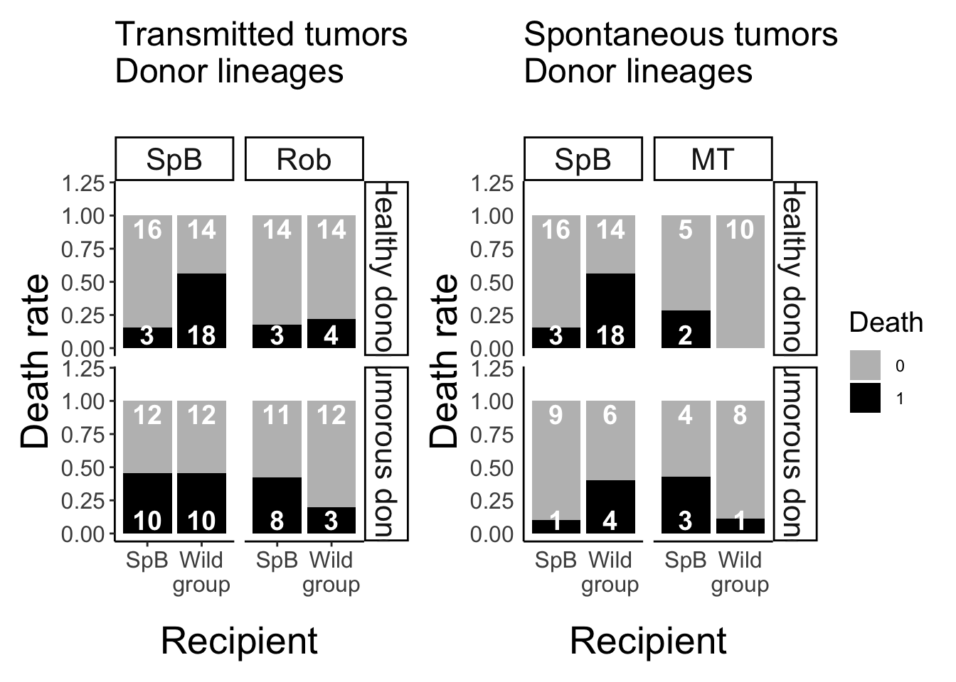
Analysis of the mortality after grafting

Transmissible tumors dataset

Random effects selection (according to Zuur et al. 2009)

mr1 <- glmmTMB(data=donor_trans, Death ~ donor * donor_status + receiver + (1|lot) + (1|date_draft), family = binomial, REML = T)
mr2 <- glmmTMB(data=donor_trans, Death ~ donor * donor_status + receiver + (1|date_draft/lot), family = binomial, REML = T)
mr3 <- glmmTMB(data=donor_trans, Death ~ donor * donor_status + receiver + (1|lot), family = binomial, REML = T)
mr4 <- glmmTMB(data=donor_trans, Death ~ donor * donor_status + receiver + (1|date_draft), family = binomial, REML = T)
mr5 <- glmmTMB(data=donor_trans, Death ~ donor * donor_status + receiver, family = binomial, REML = T)

AICc(mr1, mr2, mr3, mr4, mr5)

##     df     AICc
## mr1  7 216.6192
## mr2  7 216.6192
## mr3  6 218.7957
## mr4  6 214.4363
## mr5  5 218.2406

There is no need to include any of the potential random effects that have been measured.

Fixed effects selection

m1 <- glmmTMB(data=donor_trans, Death ~ donor * donor_status * receiver+ (1|date_draft), family = binomial, REML = F)
m2 <- glmmTMB(data=donor_trans, Death ~ donor * donor_status + receiver+ (1|date_draft), family = binomial, REML = F)
m3 <- glmmTMB(data=donor_trans, Death ~ donor + donor_status * receiver+ (1|date_draft), family = binomial, REML = F)
m4 <- glmmTMB(data=donor_trans, Death ~ donor * receiver + donor_status+ (1|date_draft), family = binomial, REML = F)

m5 <- glmmTMB(data=donor_trans, Death ~ donor + donor_status + receiver+ (1|date_draft), family = binomial, REML = F)
m6 <- glmmTMB(data=donor_trans, Death ~ donor + donor_status+ (1|date_draft), family = binomial, REML = F)
m7 <- glmmTMB(data=donor_trans, Death ~ donor + receiver+ (1|date_draft), family = binomial, REML = F)
m8 <- glmmTMB(data=donor_trans, Death ~ donor_status + receiver+ (1|date_draft), family = binomial, REML = F)

m9 <- glmmTMB(data=donor_trans, Death ~ donor * donor_status+ (1|date_draft), family = binomial, REML = F)
m10 <- glmmTMB(data=donor_trans, Death ~ donor * receiver+ (1|date_draft), family = binomial, REML = F)
m11 <- glmmTMB(data=donor_trans, Death ~ donor_status * receiver+ (1|date_draft), family = binomial, REML = F)

m12 <- glmmTMB(data=donor_trans, Death ~ donor+ (1|date_draft), family = binomial, REML = F)
m13 <- glmmTMB(data=donor_trans, Death ~ donor_status+ (1|date_draft), family = binomial, REML = F)
m14 <- glmmTMB(data=donor_trans, Death ~ receiver+ (1|date_draft), family = binomial, REML = F)

m15 <- glmmTMB(data=donor_trans, Death ~ 1+ (1|date_draft), family = binomial, REML = F)

AICc(m1, m2, m3, m4, m5, m6, m7, m8, m9, m10, m11, m12, m13, m14, m15)

##     df     AICc
## m1   9 210.4327
## m2   6 214.1003
## m3   6 208.0035
## m4   6 210.3432
## m5   5 212.4761
## m6   4 211.9316
## m7   4 211.5997
## m8   4 215.5363
## m9   5 213.4983
## m10  5 209.6024
## m11  5 210.9490
## m12  3 210.8021
## m13  3 215.4346
## m14  3 214.5699
## m15  2 214.1961

Table of the results of the best fitted models (lower AICc+2)

	Death			Death
Predictors	Odds Ratios	CI	p	Odds Ratios	CI	p
donor [Rob]	0.43	0.20 – 0.91	0.027	0.95	0.34 – 2.64	0.915
donor status [T]	4.42	1.40 – 13.91	0.011
receiver [TV]	4.38	1.41 – 13.61	0.011	2.69	1.06 – 6.83	0.037
donor status [T] × receiver [TV]	0.15	0.03 – 0.66	0.013
donor [Rob] × receiver [TV]				0.22	0.05 – 0.97	0.046
ICC	0.14			0.14
N	16 _{date_draft}			16 _{date_draft}
Observations	164			164

m10 <- glmmTMB(data=donor_trans, Death ~ donor * receiver+ (1|date_draft), family = binomial, REML = T)
tab_model(m10, show.intercept = F, show.r2 = F, show.re.var = F)

	Death
Predictors	Odds Ratios	CI	p
donor [Rob]	0.94	0.34 – 2.59	0.911
receiver [TV]	2.60	1.04 – 6.50	0.040
donor [Rob] × receiver [TV]	0.23	0.05 – 1.00	0.050
ICC	0.16
N _{date_draft}	16
Observations	164

The results are quite unclear, the best fitted models are a bit incoherent so it might just indicate a lack of power for analysis.

Spontaneaous tumors dataset

Random effects selection

m1 <- glmmTMB(data=donor_spont, Death ~ donor + receiver + donor_status + (1|lot) + (1|date_draft), family = binomial, REML = T)
m2 <- glmmTMB(data=donor_spont, Death ~ donor + donor_status + receiver + (1|date_draft/lot), family = binomial, REML = T)
m3 <- glmmTMB(data=donor_spont, Death ~ donor + donor_status + receiver + (1|lot), family = binomial, REML = T)
m4 <- glmmTMB(data=donor_spont, Death ~ donor + donor_status + receiver + (1|date_draft), family = binomial, REML = T)
m5 <- glmmTMB(data=donor_spont, Death ~ donor + donor_status + receiver, family = binomial, REML = T)

AICc(m1, m2, m3, m4, m5)

##    df     AICc
## m1  6 133.7708
## m2  6 133.7708
## m3  5 131.5171
## m4  5 131.5171
## m5  4 129.3089

There is no need to include any of the potential random effects that have been measured.

Fixed effects selection

m1 <- glmmTMB(data=donor_spont, Death ~ donor * donor_status * receiver, family = binomial, REML = F)
m2 <- glmmTMB(data=donor_spont, Death ~ donor * donor_status + receiver, family = binomial, REML = F)
m3 <- glmmTMB(data=donor_spont, Death ~ donor * receiver + donor_status, family = binomial, REML = F)
m4 <- glmmTMB(data=donor_spont, Death ~ donor + receiver * donor_status, family = binomial, REML = F)

m5 <- glmmTMB(data=donor_spont, Death ~ donor + donor_status + receiver, family = binomial, REML = F)

m6 <- glmmTMB(data=donor_spont, Death ~ donor + donor_status, family = binomial, REML = F)
m7 <- glmmTMB(data=donor_spont, Death ~ donor + receiver, family = binomial, REML = F)
m8 <- glmmTMB(data=donor_spont, Death ~ donor_status + receiver, family = binomial, REML = F)

m9 <- glmmTMB(data=donor_spont, Death ~ donor * donor_status, family = binomial, REML = F)
m10 <- glmmTMB(data=donor_spont, Death ~ donor * receiver, family = binomial, REML = F)
m11 <- glmmTMB(data=donor_spont, Death ~ donor_status * receiver, family = binomial, REML = F)

m12 <- glmmTMB(data=donor_spont, Death ~ donor, family = binomial, REML = F)
m13 <- glmmTMB(data=donor_spont, Death ~ donor_status, family = binomial, REML = F)
m14 <- glmmTMB(data=donor_spont, Death ~ receiver, family = binomial, REML = F)

m15 <- glmmTMB(data=donor_spont, Death ~ 1, family = binomial, REML = F)

AICc(m1, m2, m3, m4, m5, m6, m7, m8, m9, m10, m11, m12, m13, m14, m15)

##     df     AICc
## m1   8 122.1274
## m2   5 129.4063
## m3   5 118.0007
## m4   5 130.6583
## m5   4 129.3615
## m6   3 130.4765
## m7   3 127.3710
## m8   3 130.5674
## m9   4 130.3118
## m10  4 115.8866
## m11  4 131.6759
## m12  2 128.6919
## m13  2 131.6276
## m14  2 129.0768
## m15  1 130.4255

The best model is the m10, tacking into account the donor line and the recipient line.

	Death
Predictors	Odds Ratios	CI	p
donor [MT]	3.47	0.76 – 15.87	0.108
receiver [TV]	6.88	2.04 – 23.21	0.002
donor [MT] × receiver [TV]	0.01	0.00 – 0.19	0.001
Observations	104

The Mt donor induces more mortality in the TV recipient than in the SpB recipient.

Analysis of the mortality after grafting

Transmissible tumors dataset

Random effects selection (according to Zuur et al. 2009)

Fixed effects selection

Table of the results of the best fitted models (lower AICc+2)

Spontaneaous tumors dataset

Random effects selection

Fixed effects selection

Data visualisation